My Musings on Life

When Your Database Becomes the Bottleneck: A Practical Guide to Performance Debugging

I watched a junior developer stare at his screen last week, refreshing a page that took fifteen seconds to load. His application worked perfectly on his laptop with test data, but the moment real users started hitting the production database, everything ground to a halt. This scenario plays out in engineering teams everywhere, and it’s often the first time developers realize that writing correct SQL and writing fast SQL are entirely different skills.

Database performance issues rarely announce themselves clearly. Your application might feel sluggish during peak hours, certain pages might timeout intermittently, or you might notice your server costs creeping up as you add more instances to handle the same workload. These symptoms point to a fundamental truth: databases are often the bottleneck in your system, and understanding how to diagnose and fix performance problems is necessary for any developer building real applications.

Start with Query Execution Plans

Before you can optimize anything, you need to understand what your database is actually doing. Every major database system gives you tools to show the execution plan for your queries, and this should be your first stop when investigating slow performance. In PostgreSQL, you can prefix any query with EXPLAIN ANALYZE to see exactly how the database engine processes your request.

When I examine execution plans with new developers, I focus on three key metrics: the total execution time, any table scans happening on large tables, and whether the database is using indexes effectively. A query that scans through 100,000 rows to find 10 matching records is telling you something important about missing indexes. Similarly, a nested loop join between two large tables often indicates that you need to reconsider your query structure or add appropriate indexes.

The most valuable lesson here is learning to read the numbers. An execution plan that shows 0.1ms for the actual query but 500ms for sorting results tells you exactly where to focus your optimization efforts. This data-driven approach removes guesswork and gives you concrete evidence of what’s actually slow.

Index Strategy Beyond Primary Keys

Most developers understand that primary keys get indexed automatically, but the real performance gains come from strategic secondary indexes. I’ve seen applications transform from unusably slow to lightning fast with the addition of a single well-placed index. The key is understanding your query patterns and knowing which columns appear frequently in WHERE clauses, JOIN conditions, and ORDER BY statements.

Consider a typical user activity tracking table where you frequently query by user_id and created_at together. A composite index on (user_id, created_at) will dramatically outperform separate indexes on each column because it allows the database to eliminate rows efficiently on both criteria simultaneously. However, order matters in composite indexes. An index on (user_id, created_at) helps queries filtering by user_id alone, but won’t help queries filtering only by created_at.

The trade-off with indexes is storage space and write performance. Each index needs to be maintained whenever you insert, update, or delete rows. I typically start by adding indexes for the slowest, most frequent queries, then monitor the impact on write performance. Modern databases handle dozens of indexes on active tables without significant issues, but adding indexes carelessly will eventually hurt your write throughput.

Connection Pooling and Resource Management

Database connections are expensive resources, and connection management often becomes a performance bottleneck as applications scale. Each connection consumes memory on the database server, and most databases have limits on total concurrent connections. When your application exhausts the connection pool, new requests either fail immediately or queue up waiting for available connections.

Connection pooling solves this by maintaining a shared pool of database connections that your application can reuse. Instead of opening a new connection for each request, your application borrows a connection from the pool, executes its queries, and returns the connection for other requests to use. Popular connection poolers like PgBouncer for PostgreSQL can reduce connection overhead dramatically and allow your database to handle many more concurrent requests.

The configuration details matter here. Pool size should typically be set to match your database’s available connections divided by the number of application instances. Connection timeout settings prevent requests from waiting indefinitely for busy connections. I usually start with conservative settings and adjust based on monitoring data, watching for connection pool exhaustion or queries timing out while waiting for connections.

Query Optimization Patterns

Effective query optimization follows predictable patterns once you understand how databases process different types of operations. N+1 queries represent one of the most common performance killers in applications using ORMs. This happens when you fetch a list of records, then loop through each one making additional queries for related data. A simple blog post listing that makes one query for posts and then one query per post for the author will execute 101 queries for 100 posts.

The solution involves restructuring your queries to fetch all required data in fewer operations. JOIN operations allow you to combine related data in a single query, while techniques like batch loading can fetch related records in bulk. Most modern ORMs provide mechanisms for eager loading related data, but you need to be explicit about which relationships to include.

Pagination becomes critical as your datasets grow. Offset-based pagination using LIMIT and OFFSET works for small datasets but becomes prohibitively slow on large tables because the database still needs to process and skip all the offset rows. Cursor-based pagination using WHERE clauses with indexed columns performs consistently regardless of how deep into the dataset you paginate. This pattern scales naturally and provides better user experience for applications with large datasets.

Monitoring and Continuous Improvement

Database performance optimization is an ongoing process, not a one-time fix. Production workloads change over time as you add features, gain users, and accumulate data. Queries that performed well with 1,000 rows might become problematic with 100,000 rows. Regular monitoring helps you identify performance regressions before they impact users.

Most database systems provide built-in monitoring tools that track slow queries, index usage, and system resource consumption. PostgreSQL’s pg_stat_statements extension logs query performance statistics over time, making it easy to identify your slowest queries and track performance trends. Cloud database providers typically offer additional monitoring dashboards that surface key metrics without requiring deep database administration knowledge.

Setting up alerts for key metrics like average query execution time, connection pool utilization, and slow query frequency gives you early warning when performance starts degrading. I recommend establishing baseline measurements when your application is performing well, then alerting when metrics deviate significantly from these baselines.

Database performance optimization requires patience and systematic investigation, but the impact on user experience and system scalability makes it one of the most valuable skills you can develop. Start with understanding your current performance characteristics through execution plans and monitoring tools, then focus on the optimization techniques that address your specific bottlenecks.

Understanding Go’s Memory Management: A Gentle Introduction to the Garbage Collector

Why Go’s Memory Model Matters More Than You Think

After fifteen years of watching developers struggle with memory management across different languages, I’ve learned that understanding your runtime’s memory behavior isn’t just academic curiosity. It’s the difference between shipping code that works and shipping code that works reliably under load. Go’s garbage collector is one of the most thoughtful approaches to automatic memory management I’ve encountered, but like any sophisticated system, it rewards those who take time to understand its design principles.

Understanding Go's Memory Management: A Gentle Introduction to the Garbage Collector — Understanding Go’s Memory Management: A Gentle Introduction to the Garbage Collector

The Go runtime manages memory through a tricolor concurrent mark-and-sweep collector that has been refined through years of production use at Google and countless other organizations. What makes it particularly elegant is how it balances throughput with predictable latency, solving the classic tension that has plagued garbage-collected languages for decades. When you write Go code, you’re not just writing against the language specification. You’re writing against a memory management system that makes specific trade-offs, and understanding those trade-offs will fundamentally change how you structure your programs.

Illustration for Understanding Go's Memory Management: A Gentle Introduction to the Garbage Collector — Illustration for Understanding Go’s Memory Management: A Gentle Introduction to the Garbage Collector

The Stack and Heap: Where Your Variables Actually Live

Every Go program operates with two primary memory regions: the stack and the heap. The stack grows and shrinks automatically as functions are called and return, housing local variables that the compiler can prove won’t outlive their containing function. This is where your simple integers, small structs passed by value, and other short-lived data typically reside. Stack allocation is essentially free from a garbage collection perspective because the memory is reclaimed automatically when the function returns.

The heap, however, is where things get interesting. When the Go compiler performs escape analysis and determines that a variable might be accessed after its containing function returns, that variable “escapes to the heap.” This happens more often than newcomers expect. Taking the address of a local variable, returning a pointer to a local variable, or storing a variable in a slice that outlives the function will all trigger heap allocation. Understanding this distinction isn’t just theoretical because heap allocations create work for the garbage collector.

I’ve seen teams spend weeks optimizing algorithms when their real performance bottleneck was unnecessary heap allocations. The good news is that Go provides tools to help you see what’s happening. Running go build -gcflags="-m" will show you the compiler’s escape analysis decisions, revealing exactly which variables are being allocated on the heap and why. This single flag has saved me more debugging time than any other Go tooling feature.

How the Garbage Collector Actually Works

Go’s garbage collector operates on a tricolor marking algorithm that runs concurrently with your program. During each collection cycle, the collector marks objects as white (potentially garbage), gray (reachable but not yet processed), or black (reachable and processed). The process begins by marking all directly reachable objects from roots like global variables and stack variables as gray, then methodically processes the gray set, marking referenced objects as gray and processed objects as black.

What makes Go’s implementation particularly sophisticated is how it handles the concurrent execution challenge. Your program continues running while the garbage collector works, which means object references can change during collection. Go solves this through write barriers that track pointer modifications during the mark phase, ensuring the collector doesn’t miss newly created references or incorrectly collect objects that become reachable after marking begins.

The collector triggers automatically based on heap growth, typically running when the heap doubles in size since the last collection. This adaptive approach means that programs with steady allocation patterns develop predictable collection rhythms, while programs with bursty allocation get more frequent collection during heavy periods. You can observe this behavior in your own programs by setting GODEBUG=gctrace=1, which prints detailed information about each garbage collection cycle including duration, heap sizes, and CPU utilization.

Practical Strategies for Memory-Friendly Code

Writing Go code that works well with the garbage collector isn’t about avoiding allocations entirely. It’s about being intentional with your allocation patterns and understanding the cost implications of different approaches. One of the most effective techniques I’ve learned is object reuse through sync.Pool for frequently allocated temporary objects. This pattern is particularly valuable for things like buffer allocation in HTTP handlers or temporary data structures in hot code paths.

Another important technique is understanding slice and map growth patterns. Go slices double in capacity when they exceed their current size, which can lead to surprising memory usage if you’re not careful about pre-sizing containers. When you know the approximate final size of a slice, using make([]T, 0, expectedSize) eliminates the reallocations and copies that would otherwise occur during growth. Similarly, maps benefit from size hints when you can provide them, reducing the number of internal rehashing operations during initial population.

Pointer-heavy data structures deserve special attention because they create more work for the garbage collector during marking phases. Every pointer field in your structs is a potential reference the collector must follow. Sometimes replacing pointer fields with value types or using techniques like string interning can significantly reduce GC pressure. I’ve seen 30% garbage collection time reductions from carefully restructuring hot data types to minimize pointer chasing, though such optimizations should always be guided by actual profiling data rather than premature assumptions.

Measuring and Understanding Your Program’s Memory Behavior

The Go runtime provides exceptional tooling for understanding memory behavior, but knowing which tools to use and when makes all the difference. The built-in pprof package can generate detailed heap profiles showing allocation patterns, object counts, and memory usage by type and location. Running go tool pprof http://localhost:6060/debug/pprof/heap against a running program with the net/http/pprof handler enabled gives you a detailed view of where your program allocates memory and how much.

For development and testing, I’ve found the GOMEMLIMIT environment variable incredibly useful for understanding how your program behaves under memory pressure. Setting a memory limit forces the garbage collector to run more aggressively as you approach the threshold, helping you identify allocation hotspots and understand your program’s memory requirements under different conditions. This is particularly valuable when preparing applications for deployment in memory-constrained environments like containers.

Go’s garbage collector is designed to be a reliable partner, not an adversary. It makes reasonable default choices for most programs, but it rewards developers who understand its behavior and design their code accordingly. Start by using the escape analysis flags to understand your allocation patterns, then move on to heap profiling for the areas where performance matters most. The time invested in understanding these fundamentals pays dividends in every Go program you’ll write afterward.

If you found this introduction helpful and want to dig deeper into specific aspects of Go’s memory management, I’d love to hear about the particular challenges you’re facing in your own projects. Understanding how other developers encounter and solve memory-related problems helps me focus future writing on the areas where practical guidance can make the biggest difference.

Your First Distributed System: Start With These Three Patterns Before You Get Fancy

Why Most Engineers Pick the Wrong Starting Point

After watching dozens of teams stumble through their first distributed systems, I’ve noticed a pattern. Engineers who’ve mastered monoliths often jump straight to the sexiest distributed patterns they’ve read about: event sourcing, CQRS, microservices with complex orchestration. They build systems that look impressive in architecture diagrams but crumble under real-world load because they skipped the fundamentals.

Your First Distributed System: Start With These Three Patterns Before You Get Fancy

The truth is that distributed systems aren’t just bigger versions of single-server applications. They introduce failure modes you’ve never encountered, consistency challenges that don’t exist in monoliths, and operational complexity that can overwhelm even experienced teams. I learned this the hard way during a payment system rewrite in 2018, when our team spent six months building an elegant event-driven architecture that couldn’t handle network partitions gracefully.

Your first distributed system should teach you how distributed systems fail, not how clever you are. Start with patterns that expose you to the core challenges while remaining simple enough to reason about when things go wrong. And trust me, things will go wrong.

Pattern One: Database per Service with Eventual Consistency

Begin with two services that each own their data completely. No shared databases, no distributed transactions. Let’s say you’re building an e-commerce system. Start with a user service that manages accounts and an inventory service that tracks products. Each service gets its own database, and they communicate through HTTP APIs or message queues.

This pattern immediately teaches you about network failures, service boundaries, and data consistency challenges. When the inventory service is down, your user service keeps working, but users can’t browse products. When a user updates their shipping address while placing an order, you’ll discover that keeping related data in sync across services requires careful thought about timing and failure recovery.

Build this first because it’s the foundation of every other distributed pattern you’ll encounter. You’ll learn to think in terms of service boundaries, handle partial failures gracefully, and design APIs that don’t assume perfect network conditions. I recommend starting with just two services and gradually adding a third once you’ve experienced a few midnight pages about inconsistent state between your initial services.

The key insight you’ll gain is that perfect consistency isn’t always necessary. Users can tolerate slightly stale inventory counts, but they can’t tolerate a completely broken checkout process. This pattern forces you to think about which consistency guarantees actually matter for your business logic.

Pattern Two: Load Balancer with Health Checks

Once you understand service boundaries, add horizontal scaling to one of your services. Deploy multiple instances of your user service behind a load balancer that actively monitors instance health. This seems straightforward until you realize that “healthy” is more nuanced than “responds to HTTP requests.”

A service might respond to health checks while its database connection pool is exhausted, or while it’s experiencing memory pressure that makes it slow but not dead. You’ll learn to design health checks that actually reflect your service’s ability to handle real work, not just return a 200 status code. This means checking database connectivity, validating that critical dependencies are reachable, and sometimes even running lightweight versions of your core business logic.

This pattern teaches you about graceful degradation and the difference between hard failures and soft failures. When one instance starts returning errors because of memory pressure, how quickly does your load balancer detect this? How do you handle the case where removing a failing instance would overload the remaining healthy instances?

You’ll also discover that load balancing isn’t just about distributing requests evenly. Different requests have different resource requirements, and sticky sessions can help with caching but complicate failure recovery. Build a simple round-robin setup first, then experiment with weighted routing based on instance capacity.

Pattern Three: Circuit Breaker for External Dependencies

Now add an external dependency to one of your services. Maybe your user service needs to validate addresses through a third-party API, or your inventory service integrates with a supplier’s system. Implement a circuit breaker pattern around these external calls.

This pattern reveals how cascading failures propagate through distributed systems. When that address validation service becomes slow, does your entire user registration process grind to a halt? When the supplier API is down, should your inventory service refuse all requests, or can it operate with cached data?

A well-implemented circuit breaker monitors failure rates and response times, automatically switching to a fail-fast mode when the external service is struggling. But the real learning comes from deciding what “failure” means for each dependency and how your service should behave when operating with degraded functionality.

You’ll find yourself designing fallback mechanisms and thinking carefully about timeouts. A five-second timeout might be reasonable for a user-facing request, but catastrophic for a service handling thousands of requests per second. This pattern forces you to quantify your expectations about external dependencies and plan for their inevitable failures.

The Foundation Before the Flourishes

These three patterns form the foundation of reliable distributed systems. Database per service teaches you about data consistency and service boundaries. Load balancing with health checks introduces you to horizontal scaling and failure detection. Circuit breakers show you how to handle external dependencies gracefully.

Master these patterns before you consider more complex approaches like event sourcing, distributed consensus algorithms, or service mesh architectures. Each adds significant complexity and operational overhead that can obscure the fundamental lessons you need to learn first.

The goal isn’t to build the most sophisticated system possible. It’s to build something that works reliably and teaches you how distributed systems fail. Once you’ve experienced a few failures with these simpler patterns, you’ll have the intuition to evaluate whether more complex patterns actually solve problems you have, rather than problems you think you might have someday.

If you’re working through these patterns and hitting interesting challenges, I’d love to hear about them. The failure modes you discover in your specific domain often reveal insights that apply far beyond your immediate use case.

Production Kubernetes Deployments: Hard-Won Lessons from Five Years in the Trenches

The Evolution from Simple to Sophisticated

When we first moved to Kubernetes in production back in 2019, our deployment strategy was embarrassingly simple. We had a single cluster running in us-west-2, kubectl apply was our deployment tool, and we thought we were sophisticated because we had separate namespaces for staging and production. That setup lasted exactly three weeks before a misconfigured ingress controller brought down our entire platform during Black Friday weekend.

Production Kubernetes Deployments: Hard-Won Lessons from Five Years in the Trenches

The incident taught us that Kubernetes gives you the building blocks for resilient systems, but it doesn’t enforce good practices. You can absolutely shoot yourself in the foot with the same ease that you can build something bulletproof. The difference is understanding not just what Kubernetes can do, but what happens when those capabilities meet real-world failure scenarios.

Over the following months, we rebuilt our approach from the ground up. What emerged was a deployment strategy that prioritized observability and gradual rollouts over speed. We learned to treat every deployment as a potential failure point and design accordingly. The sophistication came not from complex tooling, but from paying attention to the basics of change management in distributed systems.

Illustration for Production Kubernetes Deployments: Hard-Won Lessons from Five Years in the Trenches

Multi-Cluster Reality and the Regional Disaster That Changed Everything

The AWS us-east-1 outage in December 2021 caught us with our pants down. We had been running a single cluster per region, thinking that was sufficient redundancy. When the entire region became unreachable for six hours, we discovered that our “disaster recovery” plan was mostly theoretical. Our monitoring lived in the same region as our application, our CI/CD pipeline couldn’t reach the cluster to assess status, and our team spent those six hours flying blind.

The post-mortem led us to a multi-cluster architecture that I initially resisted. Managing multiple clusters seemed like unnecessary complexity, but the alternative was accepting that regional outages would continue to mean complete service unavailability. We settled on a pattern of paired clusters within each region, with automatic failover handled by external DNS management. Each cluster runs identical workloads, but they’re deployed in a staggered fashion that gives us time to catch issues before they spread.

The operational overhead is real. You’re basically doubling your infrastructure surface area, and troubleshooting becomes more complex when you need to consider cluster-specific issues. But the resilience gains are substantial. During the next significant AWS event, our users experienced minor latency increases rather than complete outages. That’s the kind of improvement that makes the complexity worthwhile.

GitOps and the Deployment Pipeline That Actually Works

We’ve tried every deployment tool that’s gained traction in the Kubernetes ecosystem. Helm seemed promising until we hit the templating complexity wall around chart version 15. Kustomize felt cleaner but became unwieldy once we needed environment-specific configurations across multiple clusters. ArgoCD finally gave us the declarative approach that matched how we think about infrastructure state.

Our current GitOps setup uses ArgoCD with a multi-repository pattern that separates application configuration from deployment manifests. Application teams own their service definitions, while platform teams manage the cluster-specific configurations and policies. This separation of concerns prevents the configuration sprawl that plagued our earlier attempts. When a developer wants to change a resource limit, they modify a value in their repository, and the change flows through our environments automatically based on branch promotion.

The key insight was treating deployments as state reconciliation rather than imperative operations. Instead of thinking “deploy version 1.4.3 to production,” we think “production should be running version 1.4.3.” That mental shift eliminates entire categories of deployment issues related to partial failures and inconsistent state. ArgoCD handles the mechanics of getting from the current state to the desired state, and it’s remarkably good at dealing with the edge cases that used to require manual intervention.

Monitoring the GitOps pipeline requires different metrics than traditional deployment tools. We track sync status, drift detection, and reconciliation time rather than deployment success rates. When ArgoCD reports configuration drift, it usually means someone made manual changes that need to be either reverted or codified in git. That feedback loop has dramatically improved our configuration discipline.

Progressive Delivery and the Canary Deployments That Saved Us

The most valuable deployment capability we’ve built is progressive delivery with automated rollback. We use Flagger integrated with Istio to manage canary deployments, and it’s prevented more production incidents than any other single tool in our arsenal. The setup wasn’t trivial, but the safety net it provides has changed how confidently we can ship changes.

Our canary process starts by routing 5% of traffic to the new version while monitoring error rates, response times, and custom business metrics. If any metric crosses predefined thresholds, Flagger automatically rolls back to the previous version. The beauty is in the automation. Humans are terrible at monitoring dashboards during deployments, especially at 2 AM. Flagger never gets distracted, never decides that a small increase in error rate is “probably fine,” and never hesitates to abort a deployment that’s showing warning signs.

The metrics selection took considerable tuning. We learned that generic infrastructure metrics like CPU usage aren’t sufficient for catching application-level regressions. Our canary analysis now includes business metrics like successful payment processing rates and user session duration. These metrics often reveal issues that wouldn’t show up in traditional monitoring until much later.

The psychological impact of automated canary deployments has been as important as the technical benefits. Developers deploy more frequently because they trust the safety mechanisms. That increased deployment frequency has reduced the complexity of individual changes, creating a positive cycle of smaller, less risky deployments.

What We’ve Learned About Production Readiness

Five years of running Kubernetes in production has taught us that the technology itself is only half the equation. The other half is operational discipline, and that comes from experiencing enough failures to understand what can go wrong. Our current deployment strategy works not because it’s theoretically sound, but because it’s been hardened by real incidents and real operational pressure.

The most important lesson has been that complexity should be intentional and warranted. Every tool, every pattern, every additional layer of abstraction needs to solve a specific problem that you’ve actually experienced. We’ve removed as much tooling as we’ve added over the years, and our current setup feels sustainable in a way that our earlier attempts never did.

If you’re building deployment strategies for Kubernetes, start simple and evolve based on actual operational needs. Don’t try to solve theoretical problems with complex tooling. But when you do hit real limitations, don’t hesitate to invest in solutions that provide genuine operational improvements. The key is knowing the difference between necessary complexity and accidental complexity.

I’m curious about the deployment patterns other teams have landed on after years of production experience. The theoretical best practices rarely survive contact with real operational requirements, and I’d love to hear about the specific adaptations that have worked in different environments.

The Canary Deployment Pattern: Why It’s the Production Strategy You’re Probably Not Using (But Should Be)

The Gap Between Theory and Production Reality

After eight years of running Kubernetes in production across three different companies, I’ve watched teams struggle with the same challenge: how do you deploy changes without turning your Friday afternoon into a war room session? Most organizations default to blue-green deployments or rolling updates because they’re well-documented and feel safe. But there’s a deployment strategy that sits quietly in the shadows, one that I’ve come to rely on more than any other: the canary deployment pattern.

The beauty of canary deployments isn’t in their complexity—it’s in their surgical precision. While blue-green gives you the nuclear option of instant rollback and rolling updates provide gradual transitions, canary deployments let you test your changes against real production traffic with a level of control that feels almost surgical. You’re not gambling with your entire user base. You’re making calculated, measurable bets with a small subset of traffic while keeping the blast radius contained.

I first encountered canary deployments at a fintech startup where downtime measured in minutes translated to revenue loss measured in thousands. The traditional approaches felt too binary—either everything worked or everything broke. Canary deployments gave us something different: the ability to fail gracefully and learn step by step. That experience changed how I think about production deployments.

Building Canary Infrastructure That Actually Works

The technical implementation of canary deployments in Kubernetes requires three core components that work together: an ingress controller with traffic splitting capabilities, comprehensive observability tooling, and automated decision-making logic. Most teams get the first part right but stumble on the observability and automation pieces, which is where canary deployments either shine or become operational nightmares.

For the ingress layer, I’ve had the best results with Istio’s VirtualService resources for traffic splitting, though NGINX Ingress Controller with annotations works well for simpler setups. The key insight is that your traffic splitting needs to be granular and adjustable in real-time. Static percentage splits defined at deploy time aren’t enough. You need the ability to adjust traffic distribution based on what you’re observing. In my current setup, we start with 5% traffic to the canary, then use Prometheus metrics to automatically increase to 25%, 50%, and finally 100% based on error rates, latency percentiles, and custom business metrics.

The observability component is where most implementations fall short. You need metrics that update quickly enough to catch problems before they cascade. I’ve learned to focus on three metric categories: infrastructure health (CPU, memory, network), application performance (response times, error rates), and business impact (conversion rates, user engagement). The mistake many teams make is waiting for traditional APM dashboards that aggregate data over several minutes. By the time those show problems, you’ve already impacted real users. Instead, use high-resolution metrics with 10-15 second windows for your canary analysis.

The Automation Layer: Where Canaries Really Pay Off

Manual canary deployments are useful for learning, but automated canary analysis is where this strategy becomes transformative. The automation logic needs to be conservative by default and aggressive about rollbacks. I’ve built systems that automatically promote canary deployments when all metrics stay within defined thresholds for specific time windows, but they immediately halt promotion and roll back when any metric crosses a danger threshold.

The rollback triggers deserve special attention because they determine whether your canary deployment protects you or becomes another failure point. Error rate increases are obvious triggers, but latency degradation often provides earlier warning signals. In our current implementation, we track the 95th percentile response time and halt promotion if it increases by more than 20% compared to the stable version. We also monitor for any 5xx errors in the canary. Even a single one will pause promotion for investigation.

One pattern that’s worked well for me is the concept of “canary graduation thresholds.” Rather than promoting based purely on time windows, we require the canary to process a minimum number of requests successfully. For high-traffic services, this might be 10,000 requests. For lower-traffic services, it might be 500. This approach makes sure that your canary has actually been tested under load before you trust it with more traffic.

Real-World Lessons from Production Deployments

The first major lesson about canary deployments is that they expose problems you didn’t know existed. When you route production traffic to new code gradually, you discover edge cases that never appeared in staging environments. Database connection pool exhaustion under partial load. Memory leaks that only show up after processing specific user behavior patterns. Integration timeouts with downstream services that happen only when request patterns change slightly.

These discoveries aren’t failures of the canary deployment strategy—they’re features. The alternative is discovering these same problems during a full rollout when 100% of your users are affected. I’ve watched canary deployments catch everything from configuration errors that only affected certain user segments to performance regressions that became apparent only when processing real production data volumes.

The second lesson is about organizational discipline. Canary deployments require teams to define what “success” means before deploying, not after. You can’t implement effective automated promotion without clear success criteria. This forces conversations about acceptable error rates, performance expectations, and business impact thresholds that many teams avoid. The technical implementation pushes you toward operational maturity whether you planned for it or not.

The most surprising lesson has been about deployment frequency. Teams that implement canary deployments well tend to deploy more often, not less. The confidence that comes from controlled, observable, automatically reversible deployments changes the risk calculation entirely. Instead of batching changes into large, infrequent releases, teams start shipping smaller changes more frequently because the deployment process itself becomes less risky.

Making the Transition: Practical Next Steps

If you’re considering implementing canary deployments, start with your highest-traffic, most critical services. These services benefit most from the gradual rollout approach and provide the clearest signals for automated decision-making. Begin with manual canary deployments using simple percentage-based traffic splitting to build familiarity with the pattern before adding automation layers.

Invest in observability infrastructure before you implement canary automation. You need reliable, fast-updating metrics and alerting before you can trust automated promotion decisions. Many teams rush to automate canary deployments without the observability foundation to support good automation decisions. This leads to systems that either promote deployments too aggressively or never promote at all.

The path forward isn’t about replacing all your deployment strategies with canary patterns. Blue-green deployments still make sense for database migrations or major infrastructure changes. Rolling updates work well for stateless services where gradual replacement is sufficient. But for user-facing applications where you need to balance deployment speed with risk mitigation, canary deployments offer a middle path that I’ve found more organizations need than realize.

I’d be curious to hear about your experiences with production deployment strategies and whether canary deployments might solve challenges you’re facing. The tooling has matured significantly in the past few years, making implementation more straightforward than many teams expect.

The Distributed Systems Pattern Nobody Talks About: Why Saga Orchestration Beats Event Choreography

The Problem Hidden in Plain Sight

Three years ago, I watched a promising microservices architecture collapse under the weight of its own complexity. The team had religiously followed the event choreography pattern, publishing domain events and letting services react autonomously. On paper, it looked elegant. In production, debugging a failed payment flow meant tracing through seventeen different services, each making decisions based on events from upstream neighbors they barely understood.

The real kicker? When the customer support team called asking why a refund had processed but inventory wasn’t restored, nobody could answer. The system had become a black box of emergent behavior, and the original architects had moved on to other companies. This is when I learned that distributed systems patterns aren’t just about technical elegance. They’re about operational reality, and some patterns age much better than others.

Why Saga Orchestration Deserves Your Attention

The saga orchestration pattern sits in an interesting spot. It’s not as trendy as event sourcing or as foundational as request-response, but it solves a specific class of problems better than anything else I’ve used. Where event choreography creates implicit workflows through a chain of reactive services, saga orchestration makes the workflow explicit through a central coordinator.

Consider an order processing system. In choreography, the order service publishes an OrderCreated event. The payment service reacts by charging the card and publishes PaymentProcessed. The inventory service reacts by reserving items and publishes ItemsReserved. Each service knows only about its immediate predecessor, creating a distributed state machine that’s impossible to visualize or debug.

With saga orchestration, you have an OrderProcessingSaga that explicitly calls payment, then inventory, then shipping. When something fails at step three, the saga knows exactly what compensation actions to take. The workflow becomes code you can read, test, and modify without digging through event logs like an archaeologist.

The Netflix Example That Changed My Mind

Netflix’s approach to saga orchestration in their billing system gave me the blueprint I still follow today. They use a workflow engine called Conductor that treats each step as a task with explicit retry policies, timeouts, and compensation logic. When a subscription upgrade fails because the payment processor is down, the saga waits in a well-defined state rather than leaving the customer in limbo.

What impressed me most was their monitoring approach. Each saga execution becomes a trace you can follow from start to finish. They instrument the workflow itself, not just the individual services. This means when something breaks, you’re looking at a directed graph of what happened rather than correlating timestamps across multiple log streams.

The compensation logic is equally thoughtful. If payment succeeds but inventory allocation fails, the saga doesn’t just rollback the payment. It might queue a customer notification, create a support ticket, or trigger a backorder process. The business logic for handling partial failures lives in one place instead of being scattered across event handlers that may or may not fire reliably.

Implementation Patterns That Actually Work

Building saga orchestration requires thinking differently about service interfaces. Instead of fire-and-forget events, you need synchronous operations with clear success and failure semantics. I typically design saga steps as idempotent operations that return enough information to make compensation decisions.

The state management is important. I’ve seen teams try to build sagas with in-memory state, which works until the orchestrator crashes mid-workflow. Persisting saga state in a database with proper transactional boundaries is non-negotiable. Each step completion updates both the business state and the saga state atomically, so you never lose track of where you are in the process.

Timeout handling deserves special attention. Unlike choreography where timeouts are implicit and often ignored, saga orchestration forces you to explicitly decide what happens when a step takes too long. Some steps might retry with exponential backoff. Others might trigger manual intervention workflows. The key is making these decisions upfront rather than discovering them during outages.

The Operational Advantages Nobody Mentions

The debugging story alone makes saga orchestration worth considering. When a customer reports a problem, you can pull up their specific saga execution and see exactly what happened. Did payment fail? Did inventory allocation time out? Was there a retry loop that eventually succeeded? The answers are there in the workflow trace, not scattered across multiple service logs.

Performance monitoring becomes more meaningful too. Instead of tracking individual service metrics in isolation, you can measure end-to-end workflow performance. How long does the complete order processing saga take? Which steps are the bottlenecks? Where do most failures happen? These business-level metrics often matter more than technical metrics like CPU utilization.

The testing story improves dramatically. You can write integration tests that exercise complete workflows without setting up elaborate event choreography scenarios. Mock the individual steps and test the orchestration logic in isolation. When you do need to test with real services, the explicit workflow makes it clear what success and failure paths to cover.

When Orchestration Isn’t the Answer

Saga orchestration shines for business processes with clear start and end points, but it’s not a universal solution. High-frequency data processing pipelines often benefit more from choreography patterns where latency matters more than workflow visibility. Simple CRUD operations don’t need the overhead of explicit orchestration.

The pattern also introduces a coordination bottleneck. The saga orchestrator becomes a critical component that needs its own scaling and reliability considerations. I’ve learned to design orchestrators as lightweight coordinators that delegate actual work to other services rather than becoming monolithic workflow engines.

Consider whether your team has the operational maturity to manage explicit workflows. Choreography fails gracefully by default. Individual services might miss events, but the system keeps running. Orchestration fails explicitly, which can be better for correctness but requires more sophisticated error handling and recovery procedures.

The next time you’re designing a multi-step business process, think about whether making the workflow explicit might serve you better than hoping emergent behavior will remain predictable. Sometimes the less fashionable pattern turns out to be the one that actually solves your problem.

Go’s Memory Management Gets More Right Than Wrong

The Garbage Collector Nobody Talks About

I’ve spent the better part of a decade watching Go’s garbage collector evolve from something that would routinely pause your application for 100+ milliseconds to the remarkably predictable system we have today. The transformation has been quiet, methodical, and honestly doesn’t get the recognition it deserves from most developers who just expect their memory to be managed without thinking about it.

Go's Memory Management Gets More Right Than Wrong — Go’s Memory Management Gets More Right Than Wrong

Go’s current tricolor concurrent mark-and-sweep collector is the result of years of careful engineering. The old stop-the-world collectors from early Go? Gone. Today’s implementation runs alongside your application threads and keeps pause times under 1 millisecond for most workloads. This isn’t marketing speak. I’ve measured it across production systems handling millions of requests daily.

The tricolor algorithm works by marking objects as white (potentially unreachable), grey (reachable but not yet scanned), or black (reachable and scanned). The collector starts from root objects and propagates through the object graph, eventually freeing white objects that remain unmarked. What makes Go’s implementation special is how it handles the write barrier during concurrent marking, making sure that newly allocated objects during collection cycles don’t get incorrectly freed.

Illustration for Go's Memory Management Gets More Right Than Wrong — Illustration for Go’s Memory Management Gets More Right Than Wrong

Stack vs Heap: Where Go Makes Smart Decisions

Go’s escape analysis deserves way more credit than it gets. The compiler does sophisticated analysis to figure out whether variables can live on the stack or must be allocated on the heap. This decision completely changes both performance and garbage collection pressure, but most developers have no idea how it works.

Variables that escape to the heap usually do so for predictable reasons: they’re returned from functions, assigned to interface values, or their addresses are taken and stored in heap-allocated structures. The compiler plays it safe, sometimes allocating to the heap when stack allocation might have worked. I’ve seen cases where refactoring code to avoid unnecessary escapes reduced GC pressure by 40%.

Stack allocation in Go is incredibly efficient because stacks are segmented and growable. When a goroutine’s stack runs out of space, the runtime allocates a new, larger stack and copies the existing data. This happens behind the scenes, but understanding it helps explain why Go can spawn millions of goroutines without exhausting memory. Each goroutine starts with a 2KB stack that grows as needed, a design choice that balances memory efficiency with performance.

The GOGC Tuning Game Everyone Plays Wrong

The GOGC environment variable controls when garbage collection triggers, but I consistently see teams either ignoring it completely or setting it to random values without understanding what happens next. GOGC is the percentage of heap growth that triggers the next collection cycle. The default value of 100 means the collector runs when the heap doubles in size since the last collection.

Setting GOGC higher reduces collection frequency but increases memory usage and potentially pause times. Setting it lower does the opposite. I’ve found that most long-running services work better with values between 50 and 200, depending on their allocation patterns and memory constraints. Services with steady-state memory usage often perform better with higher GOGC values, while applications with bursty allocation patterns need more frequent collections.

Here’s the thing: GOGC tuning should be driven by actual measurements, not gut feelings. Go’s runtime gives you detailed GC statistics through debug.ReadGCStats() and the GODEBUG environment variable. I’ve seen teams achieve 20% performance improvements just by monitoring their allocation patterns and adjusting GOGC accordingly.

Memory ballasting is controversial but can be effective for applications with predictable memory usage. By allocating a large chunk of memory that never gets used, you can effectively increase the heap size baseline, reducing collection frequency. This technique works because the GC triggers based on heap growth percentage, not absolute size.

Finalizers and Weak References: The Sharp Edges

Go’s runtime.SetFinalizer gives you a mechanism for cleanup when objects become unreachable, but it’s a tool that demands respect. Finalizers run in a separate goroutine after garbage collection, with no guarantees about timing or order. They can resurrect objects, create reference cycles, and seriously complicate the collector’s job.

I’ve debugged applications where excessive finalizer usage caused memory leaks because finalizers themselves prevented objects from being collected. The finalizer queue can become a bottleneck, particularly in applications that allocate many objects requiring cleanup. The runtime has to track finalized objects separately, adding overhead to both allocation and collection.

Go doesn’t have weak references, and that’s a deliberate design choice. It occasionally frustrates developers coming from other languages. Weak references would complicate the garbage collector and the memory model significantly. Instead, Go pushes you toward explicit lifecycle management through context cancellation and cleanup functions.

Memory Allocator Internals: Beyond the Basics

Go’s memory allocator builds on TCMalloc concepts but adapts them for garbage-collected environments. The allocator uses size classes to reduce fragmentation, with separate handling for small objects (less than 32KB), large objects, and tiny objects (less than 16 bytes). Understanding these categories helps explain allocation performance characteristics.

Small object allocation uses a hierarchical approach: thread-local caches (mcache) for lock-free allocation, central caches (mcentral) for refilling thread caches, and a global heap (mheap) as the ultimate source. This design minimizes lock contention while maintaining reasonable memory efficiency. Each thread cache contains spans of memory pages organized by size class.

Large object allocation bypasses the size class system entirely, allocating directly from the global heap. These allocations cost more but happen less frequently in well-designed applications. The runtime tracks large objects separately for garbage collection, scanning them directly rather than through size class spans.

The relationship between Go’s allocator and the operating system involves careful management of virtual memory. Go requests memory from the OS in large chunks and manages it internally, releasing memory back to the OS during garbage collection when possible. The GOMEMLIMIT environment variable, introduced in Go 1.19, gives applications a soft memory limit, helping the garbage collector make better decisions about when to return memory to the OS.

After years of working with Go’s memory management across all kinds of production environments, I’m convinced that understanding these internals pays off. The abstractions work well for most use cases, but when performance matters or you’re debugging memory issues, knowing how the machinery operates makes all the difference. If you’ve had different experiences with Go’s memory management or found effective tuning strategies, I’d be interested to hear about them.

Building Your First CI/CD Pipeline: Start Simple, Scale Smart

Why Your First Pipeline Should Bore You to Tears

After watching dozens of teams stumble through their first continuous integration attempts, I’ve learned that the most successful pipelines start embarrassingly simple. The urge to build something impressive right out of the gate is natural, but it’s also the fastest way to create a system nobody understands or trusts. Your first pipeline should do exactly three things: run your tests, build your artifacts, and deploy to a single environment. That’s it.

Building Your First CI/CD Pipeline: Start Simple, Scale Smart

The beauty of this approach isn’t just simplicity. When you strip away the complexity, you can focus on getting the fundamental mechanics right. You’ll learn how your build system behaves under different conditions. You’ll understand the actual deployment dependencies. Most importantly, you’ll develop confidence in the process. I’ve seen teams spend months debugging elaborate multi-stage pipelines when their real problem was a basic configuration issue that would have been obvious in a simpler setup.

Think of your first pipeline as scaffolding, not architecture. It exists to support you while you build something more substantial. The goal is establishing a reliable foundation that your team can understand completely. Every feature you add later builds on this foundation, so make it solid and predictable. When something breaks (and it will), you want to know exactly where to look.

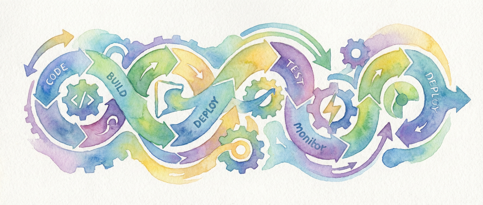
Illustration for Building Your First CI/CD Pipeline: Start Simple, Scale Smart

The Three-Stage Foundation That Actually Works

Every reliable pipeline I’ve built or inherited follows the same basic pattern: test, build, deploy. This isn’t revolutionary thinking, but the implementation details matter enormously. Your test stage should run fast and fail early. Keep your unit tests here, along with any linting or static analysis that can catch obvious problems. Save the integration tests for later stages or separate pipelines entirely. Speed matters more than completeness in this first gate.

The build stage creates deployable artifacts. Whether that’s Docker images, compiled binaries, or packaged applications depends on your stack, but the principle remains the same. Build once, deploy many times. Tag your artifacts with both the commit hash and a human-readable version number. You’ll thank yourself for this when you’re troubleshooting a deployment three months from now, trying to figure out exactly what code is running where.

Deployment should be the most boring part of your entire pipeline. By the time you reach this stage, you should have high confidence that your artifact works. Keep your deployment scripts simple and idempotent. If something fails, you should be able to run the deployment again without causing problems. This means checking if resources already exist before creating them, and handling partial deployments gracefully.

The secret sauce in this three-stage approach is what happens between stages. Each stage should produce clear, actionable feedback. Failed tests tell you exactly which test broke and why. Failed builds point to specific compilation errors or missing dependencies. Failed deployments indicate whether the problem is infrastructure, configuration, or the application itself. No guesswork required.

Configuration That Won’t Bite You Later

The biggest trap in pipeline configuration is treating it like application code. It’s not. Pipeline configuration needs to be more conservative, more explicit, and more predictable than your application. Avoid clever abstractions and dynamic behavior that seemed like good ideas at the time. Your future self, debugging a failed deployment at 2 AM, will appreciate straightforward configuration over elegant brevity.

Environment variables are your friend, but organize them thoughtfully. Create clear naming conventions that indicate scope and purpose. Database connection strings should obviously be different from API keys, and your naming should reflect that. Use a secrets management system from day one, even if it feels like overkill. Moving secrets from environment variables to proper secret management later is painful and error-prone. Trust me on this one.

Version control everything, including your pipeline configuration itself. This seems obvious until you realize how many teams keep their CI/CD scripts in a separate repository. Or worse, they edit them directly in their CI system’s web interface. Your pipeline configuration should live alongside your application code, versioned and reviewed like any other system component.

Document your configuration choices, especially the non-obvious ones. Why did you choose that particular base image? Why does the deployment script wait thirty seconds between steps? These decisions make sense when you make them. Six months later, they look arbitrary and potentially wrong. Save your future teammates the archaeology expedition. They’ll have enough real problems to solve.

Monitoring and Feedback Loops You’ll Actually Use

Building a pipeline is easy. Building a pipeline that people trust and use effectively requires thoughtful monitoring and feedback mechanisms. Start with the basics: track build success rates, deployment frequency, and time to deploy. These metrics tell you whether your pipeline helps or hinders your team’s productivity. If deployments take longer or happen less frequently after implementing CI/CD, something is wrong.

Notification fatigue kills CI/CD adoption faster than any technical problem. Be selective about what generates alerts and who receives them. Failed tests on feature branches probably don’t need to notify the entire team. Failed deployments to production definitely do. Create different notification channels for different types of events. Give people control over what they subscribe to.

The most valuable feedback comes from making pipeline status visible and accessible. Dashboard screens showing current build status, recent deployment history, and system health give teams situational awareness without requiring active monitoring. When something goes wrong, people should be able to see what happened and when, without diving into log files or CI system interfaces.

Build in mechanisms for gradual improvement. Add simple metrics collection that can help you identify bottlenecks and pain points. Track which tests fail most frequently, which stages take the longest, and where manual intervention is still required. This data becomes invaluable when you’re ready to optimize and expand your pipeline capabilities. But don’t optimize prematurely. Let real usage patterns guide your improvements.

Growing Beyond Your First Pipeline

The transition from a working pipeline to a sophisticated deployment system happens gradually. That’s exactly how it should be. Each addition should solve a specific problem your team is actually experiencing, not a problem you think you might have someday. Add staging environments when manual testing becomes a bottleneck. Implement parallel testing when your test suite grows too slow. Introduce deployment strategies like blue-green or canary releases when zero-downtime deployments become necessary.

Pay attention to the human factors as your pipeline evolves. The most technically impressive CI/CD system is worthless if your team doesn’t understand how to use it or trust it to work correctly. Changes should improve the developer experience, not complicate it. If people start avoiding the pipeline or working around it, you’ve optimized for the wrong things. I’ve made this mistake more times than I’d like to admit.

Remember that pipeline design is ultimately about reducing cognitive load and increasing confidence. Every feature should make it easier for your team to ship reliable software, not harder. The best pipeline is one that disappears into the background, handling the mechanical aspects of software delivery so your team can focus on building great products. When your pipeline works so well that nobody thinks about it, you’ve succeeded.

If you’re just starting your CI/CD journey, I’d love to hear about the specific challenges you’re facing. The implementation details that seem obvious to someone who’s built dozens of pipelines can be genuinely puzzling when you’re encountering them for the first time. Feel free to reach out with questions about your particular setup or environment. Sometimes an outside perspective can spot the simple solution you’ve been missing.

The Three Database Performance Lies That Keep Killing Production

The Index Obsession Is Destroying Your Query Plans

I’ve watched teams create index after index, believing more coverage equals better performance. This cargo cult optimization comes from a basic misunderstanding of how query planners actually work. The truth is that excessive indexing often makes your database slower, not faster.

When you have fifteen indexes on a table, the query planner spends way too much time evaluating options before choosing what’s often a suboptimal path. I’ve seen PostgreSQL choose a nested loop over a hash join because it got distracted by an index that only covered part of the WHERE clause. The planner’s cost estimates become unreliable when it’s drowning in choices.

What’s worse is the write amplification. Every INSERT becomes a small nightmare of index maintenance. I once debugged a system where bulk loads took six hours instead of thirty minutes because someone had created “helpful” indexes on every column that appeared in a WHERE clause somewhere in the application. The database spent more time maintaining indexes than actually storing data.

The solution isn’t to avoid indexes entirely, but to be ruthlessly selective. Start with your most frequent queries and work backward. Use tools like pg_stat_user_tables to see which indexes are actually being used. Drop the ones that aren’t. Your database will thank you with faster writes and more predictable query plans.

Caching Layers Are Band-Aids on Architectural Wounds

Redis sitting in front of your database became the default solution for performance problems. It’s also one of the most expensive mistakes teams make, both in complexity and actual cost. Caching feels like a silver bullet until you realize you’ve just moved the problem up a layer.

The basic issue with cache-first thinking is that it treats symptoms instead of causes. If your database queries are slow, adding a cache means you now have two systems to monitor, debug, and scale. Cache invalidation becomes a distributed systems problem. Your application logic gets polluted with cache-warming strategies and fallback mechanisms.

I’ve seen production systems where the cache layer consumed more resources than the database itself. Teams spent weeks debugging cache coherency issues that wouldn’t exist if they’d just optimized their original queries. The cache-aside pattern sounds simple until you’re dealing with thundering herds and cold starts at 3 AM.

Before reaching for Redis, exhaust your database optimization options. Proper indexing, query rewriting, and connection pooling often eliminate the need for caching entirely. When you do need a cache, make it targeted and temporary. Design for cache misses, not cache hits. Your future self will appreciate the simpler architecture when things inevitably break.

Connection Pooling Configuration Matters More Than You Think

Most teams treat connection pooling as a set-and-forget configuration detail. They pick some reasonable-sounding numbers, deploy to production, and wonder why their database still struggles under load. Connection pool tuning is where the rubber meets the road for database performance, and the default settings are almost never correct for your workload.

The pool size sweet spot is narrower than most people realize. Too few connections and you’re artificially limiting throughput. Too many and you’re creating contention at the database level. PostgreSQL performs best with connections roughly equal to your CPU cores, maybe double if you have a lot of I/O wait. But that’s just the starting point.

Connection lifetime management is equally important. I’ve debugged systems where connections were being churned every few seconds, overwhelming the database with authentication overhead. On the flip side, I’ve seen connections held open for hours, tying up resources and preventing proper load distribution. The solution is understanding your application’s actual connection patterns, not just guessing.

Modern poolers like PgBouncer offer different pooling modes for different scenarios. Session pooling for applications that need transaction guarantees, transaction pooling for stateless workloads, and statement pooling for maximum efficiency with simple queries. Choose the wrong mode and you’ll either break your application or leave performance on the table. Measure your connection utilization patterns before making these decisions.

Query Optimization Requires Understanding Data Distribution

The most elegantly written query can perform terribly if you don’t understand how your data is distributed. Query planners make decisions based on statistics, and when those statistics don’t reflect reality, even perfect indexes won’t save you.

Consider a user table where 90% of records have a status of ‘active’ but your query filters for ‘inactive’ users. The planner might choose a full table scan because its statistics suggest the filter isn’t selective enough to warrant an index lookup. But if you’re specifically looking for that 10% minority case, you want the index every time.

Data skew problems get worse over time. A table that started with even distribution might develop hot spots as the application evolves. I’ve seen systems where queries ran fine for months until a particular customer’s data volume crossed a threshold, turning a previously efficient nested loop into a performance killer.

Regular statistics updates help, but they’re not magic. Use ANALYZE frequently on rapidly changing tables. For PostgreSQL, consider increasing the statistics target for columns with high cardinality or unusual distributions. Sometimes you need to hint the planner with targeted partial indexes or even resort to query restructuring to work with the statistics you have, not the statistics you wish you had.

The Real Work Happens in Production

Database performance optimization is ultimately an empirical discipline. You can follow all the best practices, read every blog post, and still miss the specific quirks of your workload. The database doesn’t care about your architectural purity or your testing environment’s results.

What works is methodical measurement, targeted changes, and honest assessment of results. Keep detailed performance baselines. Change one thing at a time. Accept that some optimizations will fail and be prepared to roll them back quickly.

I’m curious about your own database optimization war stories. What performance assumptions have blown up in your face? What unconventional solutions have worked in your specific context? The comment section is open for sharing those hard-won lessons that only come from production experience.

The Index Cargo Cult: Why Your Database Performance Problems Run Deeper Than Missing Indexes

The Reflexive Index Solution

I’ve watched countless teams perform the same ritual when their application starts crawling: they fire up their monitoring dashboard, spot slow queries, and immediately start slapping indexes on every column that appears in a WHERE clause. It’s the database equivalent of turning it off and on again. The problem is that this reflexive response often hides deeper architectural issues while creating new problems that won’t surface until months later when your write performance has tanked so badly your application feels like it’s running underwater.

The Index Cargo Cult: Why Your Database Performance Problems Run Deeper Than Missing Indexes

Here’s what most people don’t want to hear: most performance problems aren’t solved by indexes. They’re solved by understanding data access patterns, query execution plans, and the fundamental mismatch between how developers think about data and how databases actually work. I’ve seen production systems with over 200 indexes on tables with fewer than 50 columns. Each index was added by a developer who was certain they’d found the magic fix. The result? A system that could execute any conceivable SELECT statement in milliseconds but took several seconds to complete a simple INSERT.

The Write Performance Death Spiral

Every index you add is a promise to the database engine that you’ll maintain sorted data structures for every modification. Insert a row? Every index on that table needs updating. Update a column that’s part of an index? The database has to potentially restructure B-tree nodes. Delete a row? Every index needs to remove references. This isn’t theoretical overhead. It’s measurable, cumulative, and often the actual source of performance problems that teams blame on everything except their indexing strategy.

I once inherited a system where a transaction table had 47 indexes. Forty-seven! The development team had been adding indexes for three years, each time a new query appeared slow. Insert performance had degraded by 80% over that period, but because inserts happened asynchronously in background jobs, nobody connected the dots. The system was spending more time maintaining indexes than processing actual business logic. We removed 39 of those indexes, carefully analyzing which queries would be affected. Insert performance improved by 400% while only three queries showed measurable degradation.

The lesson isn’t that indexes are bad. It’s that they’re tools with specific costs, and those costs add up in ways that aren’t always obvious. Every index is a bet that the query performance gain outweighs the write performance penalty. Most teams never revisit those bets as their application changes.

Query Pattern Analysis Over Symptom Treatment

Real database optimization starts with understanding your actual workload, not your perceived workload. I spend more time analyzing query execution plans and monitoring actual database activity than I do reading documentation or Stack Overflow posts. The pg_stat_statements extension in PostgreSQL gives you a forensic-level view of what your database is actually doing, not what you think it’s doing. Most performance problems become obvious once you see which queries are eating the most cumulative time.

Take the classic N+1 query problem that every web developer hits eventually. You can index your way out of the immediate pain, but you’re still executing hundreds of individual queries when you should be executing one. I’ve seen applications with beautifully optimized individual queries that perform terribly because they’re executing the same query pattern thousands of times per request. The solution isn’t better indexes. It’s better query design through joins, subqueries, or changing how the application fetches data.

The most effective optimizations I’ve implemented have been query rewrites that eliminated entire categories of database round trips. Replacing EXISTS subqueries with JOINs where appropriate, using window functions instead of correlated subqueries, or restructuring complex WHERE clauses to work better with index scan patterns. These changes often provide 10x performance improvements where adding indexes might give you 2x at best.

Hardware Reality and Logical Design Misalignment

Database engines are sophisticated pieces of software, but they’re constrained by physics. Disk I/O patterns matter more than most developers realize. A query that looks elegant in SQL might translate to random disk seeks that destroy performance on traditional storage, while a seemingly clunky query that accesses data sequentially runs incredibly fast. Understanding these mechanics changes how you approach schema design and query optimization.

I’ve seen teams spend thousands of dollars upgrading to NVMe storage to solve performance problems that were actually caused by poor clustering decisions. Your primary key choice affects how your data is physically stored, which affects how efficiently range scans and joins perform. A UUID primary key might satisfy your application’s requirements for globally unique identifiers, but it guarantees that every insert will cause random I/O as the database maintains sorted order. Sequential keys, despite their theoretical drawbacks, often provide measurably better performance for write-heavy workloads.

The buffer pool hit ratio is another metric that tells you whether your performance problems are CPU-bound or I/O-bound. If you’re consistently hitting disk for data that should be cached, you either need more memory or you need to restructure your queries to access data more efficiently. Throwing more CPU at an I/O-bound problem won’t help, just as adding more memory won’t solve CPU-intensive query execution.

Measurement Over Intuition

The most dangerous phrase in database optimization is “that should be fast.” I’ve learned to trust execution plans and timing data over intuition every single time. A query that looks simple might be performing a nested loop join over millions of rows, while a complex-looking query with multiple CTEs might execute in milliseconds because it’s using efficient hash joins and index scans.

Proper benchmarking requires understanding your specific workload under realistic conditions. Synthetic benchmarks running against empty tables tell you nothing about production performance with millions of rows, concurrent connections, and mixed read/write workloads. I always benchmark optimization changes under load that simulates actual usage patterns, measuring not just query execution time but also system resource utilization and impact on concurrent operations.

The feedback loop between measurement and optimization is where real expertise develops. You make a change, measure the impact across multiple metrics, and build intuition about what works in your specific environment. This experiential knowledge is what separates competent database administrators from developers who copy solutions from blog posts without understanding the tradeoffs.

Database performance is a discipline that rewards methodical analysis over quick fixes. If you’re struggling with similar issues or have war stories from your own optimization battles, I’d love to hear about the approaches that have worked in your environment. The best solutions often emerge from understanding the specific constraints and access patterns of individual systems rather than applying generic best practices.